The combination of trend-following and volatility scaling is one of the most robust edges in systematic trading. But the way most practitioners implement the volatility side is flawed in ways that matter, and a recent paper from BlackRock’s AI Lab shows a cleaner path.
Thanks for reading Algorithmic Token! Subscribe for free to receive new posts and support my work.
The Concept
Momentum is among the most replicated findings in empirical finance. Assets that have performed well over a lookback window of roughly one to twelve months tend to continue performing well over the next month. This holds across equities, futures, FX, and commodities. The underlying mechanism is debated — behavioral explanations (underreaction, herding), structural ones (trend-following flows creating their own continuation) — but the empirical regularity itself is not seriously in dispute.
Volatility targeting is the natural complement. If you size your momentum position proportional to the signal but inversely proportional to recent volatility, you achieve two things at once: the strategy allocates more aggressively in calm markets where conviction is cheaper, and it deleverages automatically before and during turbulent periods when signals are noisiest and drawdowns most painful.
Together, the combination produces something that neither approach achieves alone: a strategy with trend-following upside, substantially lower drawdowns than unscaled momentum, and a more stable risk profile across market regimes. The academic literature has documented Sharpe ratio improvements of 0.2–0.4 from adding volatility targeting to momentum strategies, with the improvement most visible in tail risk reduction.
“Volatility targeting does not improve returns. It improves the ratio of returns to risk — and it does so precisely when you most need it to.”
The practical question is not whether to volatility-target. It is how. And here is where most implementations fall short.
Source: Gemini Nanobanana Image Generation based on the Blog title and the research paper.
The Research Basis
The foundational empirical work on volatility targeting is Moreira and Muir (2017), who demonstrated that scaling portfolio exposure inversely with a variance forecast improves Sharpe ratios across asset classes and reduces tail risk without a commensurate reduction in expected returns. Their mechanism is simple: when variance is high, expected returns do not rise proportionally to compensate, so reducing exposure during high-variance periods is a free improvement in risk-adjusted terms.
This result has been confirmed across dozens of follow-on studies. But the implementation it suggests — the open-loop approach — has well-documented practical problems. A paper published in March 2026 from BlackRock’s AI Lab makes these problems precise and proposes a better solution.
Devanathan, Rueter, Boyd, Candès, Hastie, Kochenderfer, Apoorv, Soronow, Zamkovsky — BlackRock AI Lab & BlackRock Index Services · arXiv:2603.01298 · March 2026
The paper’s authors frame volatility targeting as what it really is: a control theory problem. You have a target (the volatility setpoint), an output (realized portfolio volatility), and a control input (the portfolio weight). The standard approach sets the control input purely as a function of a volatility forecast — open-loop, no feedback. The feedback control version continuously corrects for the gap between where realized volatility is and where you want it to be.
The distinction matters more than it might initially appear.
The BlackRock paper treats these as symptoms of a single underlying cause: the absence of feedback. Their proposed fix is a proportional controller — borrowed directly from classical control theory — that adjusts the weight not just based on the variance forecast but based on the gap between current realized volatility and the target.
Strategy Logic
Step 1 — The Momentum Signal
We use a time-series momentum signal over a 12-month lookback with a 1-month skip (to avoid short-term reversal contamination). The signal is the sign of the excess return over the lookback window, scaled by an estimate of signal strength.
MOMENTUM SIGNAL:
A positive signal means we take a long position in the asset; negative means short (or flat, for long-only implementations). The magnitude of the signal scales our base exposure before volatility adjustment.
Step 2 — The Volatility Target
Set a target annualised volatility, σ*. For a single-asset strategy, 10–15% annualised is typical. For a multi-asset portfolio of volatility-targeted positions, you can set each leg lower and let diversification do the work.
Step 3 — The Open-Loop Weight (baseline)
Standard (open-loop) position size:
Step 4 — The Feedback Correction (the BlackRock improvement)
The proportional controller adds a correction term based on the tracking error — the difference between the target volatility and the most recent realized volatility:
PROPOTIONAL CONTROL ADJUSTMENT:
K_p is the proportional gain — an interpretable parameter controlling how aggressively the controller corrects tracking error. Higher values mean tighter vol targeting but potentially more turnover. The clip enforces the leverage constraint: no shorting (for long-only) and a hard cap on maximum leverage.
This is the core of the paper’s contribution. The weight adjustment is no longer purely a function of a forecast — it is also a function of observed performance. If the strategy has been running above target volatility, the controller trims exposure regardless of what the forecast says. If it has been running below, the controller adds exposure. The mechanism is self-correcting.
A Note on These Strategy Labs
This is the first Strategy Lab post from our publication Algorithmic Token. With these Strategy Labs we are aiming to have a first implementation of a trading strategy pseudo-code framework, that would conditioned on feedback and positive backtests results, be further developed into proper functional production code. The pseudo-codes generated here are obviously based on the papers we have read and analyzed, and where we have found a way for a potential trading strategy implementation. The interested readers may find here their own ideas, and we encourage feedback on the comments sections or through direct email messages from those readers, about possible additions or improvements to the pseudo-codes.
Pseudocode Implementation
# Strategy Lab #1 — Momentum + Adaptive Volatility Control
# Experimental prototype — see risk disclosure

import numpy as np
import pandas as pd

def compute_momentum_signal(prices, lookback=252, skip=21):
    """
    Time-series momentum: return over [t-lookback, t-skip]
    Normalised by long-run volatility to make it comparable across assets
    """
    log_returns = np.log(prices).diff()
    raw_signal = log_returns.rolling(lookback - skip).sum().shift(skip)
    long_vol = log_returns.rolling(lookback).std() * np.sqrt(252)
    return raw_signal / long_vol  # scaled signal


def realized_vol(returns, window=21):
    """Annualised realised volatility over trailing window"""
    return returns.rolling(window).std() * np.sqrt(252)


def adaptive_vol_weight(signal, realized, target_vol=0.10,
                         Kp=0.5, w_min=0.0, w_max=1.5):
    """
    Combine momentum signal with proportional-control vol targeting.

    Kp : proportional gain (0.3–0.8 is a reasonable starting range)
    w_min/w_max : leverage constraints
    """
    # Open-loop weight from volatility forecast
    w_ol = np.sign(signal) * (target_vol / realized)

    # Tracking error: how far are we from the target?
    tracking_error = target_vol - realized

    # Proportional correction
    w_correction = Kp * (tracking_error / target_vol)

    # Final weight with leverage constraints
    w_final = np.clip(w_ol + w_correction, w_min, w_max)
    return w_final


# --- Main loop (single asset, daily bar data) ---

# prices: pd.Series of daily close prices
# Assumes transaction costs handled externally

returns = prices.pct_change()
signal  = compute_momentum_signal(prices)
rvol    = realized_vol(returns)

weights = adaptive_vol_weight(
    signal, rvol,
    target_vol=0.10,   # 10% annualised vol target
    Kp=0.5,            # moderate proportional gain
    w_min=0.0,         # no shorting (long-only)
    w_max=1.5          # max 1.5x leverage
)

strategy_returns = weights.shift(1) * returns  # avoid look-ahead
Thanks for reading Algorithmic Token! Subscribe for free to receive new posts and support my work.
Backtest Sketch
The following assumptions underpin any realistic test of this strategy. They are stated explicitly because the gap between "this looks good in simulation" and "this works in practice" lives almost entirely in the assumptions.
01 Universe: Developed market equity indices as futures (S&P 500, Euro Stoxx 50, Nikkei 225, FTSE 100). Futures avoid dividend treatment issues and provide natural leverage without margin complexity.
02 Data period: 2005–2024, covering at least two full volatility regimes (2008–09 crisis, 2020 shock) and extended low-volatility periods (2013–2019).
03 Transaction costs: Round-trip cost of 5bps per trade (futures) plus 2bps slippage. Realistic for institutional size; retail implementations should use 10–15bps. Daily rebalancing at these costs will erode returns substantially — weekly rebalancing is the practical baseline.
04 Rebalancing: Weekly, at close. Daily rebalancing is viable with the feedback controller (one of its advantages is that small corrections reduce the need for large daily trades) but costs must be modelled explicitly.
05 Proportional gain calibration:K_p should be calibrated on a holdout set, not on the test period. The paper demonstrates that the optimal gain is relatively stable across assets and periods — values in the 0.3–0.7 range tend to work well — but it must not be fitted to the backtest.
What to expect: the standard open-loop implementation will show strong Sharpe improvement versus buy-and-hold (roughly 0.6–0.9 Sharpe on individual index futures over 2005–2024). The feedback-controlled version should show marginally lower but more consistent Sharpe, meaningfully lower turnover, and substantially less frequent leverage spikes — particularly relevant during volatility regime transitions in 2018, 2020, and 2022.
Tradability assessment
Data access —------------------- 9/10
Implementation complexity —----------------- 7/10
Strategy novelty —--------------- 6/10
Data access is excellent — index futures data is widely available via Interactive Brokers, Norgate, or any futures data vendor. Implementation complexity is moderate — the feedback controller adds one parameter and a handful of lines of code, but calibrating K_p properly requires a validation framework. Strategy novelty scores lower because momentum + vol targeting is well-documented; the value here is the feedback control improvement, which is genuinely new and practically significant but not a paradigm shift.
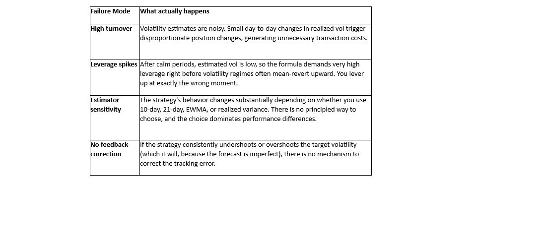
What Could Break This
Honesty about failure modes is not a disclaimer. It is the most useful part of any strategy analysis. Here are the specific ways this strategy can and does fail:
↯Momentum crashes. The most dangerous scenario for trend-following is a sharp, sustained reversal after an extended trend — October 2008, March 2020 recovery, the 2022 bond unwind. The volatility targeting reduces but does not eliminate these losses. In 2020 specifically, vol targeting actually increased equity exposure into the February drawdown because prior realized vol was low.
↯Vol targeting perversely amplifies leverage spikes in transitions. As the BlackRock paper notes, after sustained low-volatility periods, the formula demands high leverage right as regimes shift. The proportional controller partially addresses this but cannot eliminate it — it can only reduce the magnitude of the spike, not its timing.
↯Parameter stability of K_p over long horizons. The proportional gain is presented as a robust, near-universal parameter in the paper. In simulation, this holds. In live trading across structural breaks (pre/post-2008, pre/post-2020 monetary regime), gain stability should be monitored and the controller re-calibrated if tracking error trends upward persistently.
↯Crowding. Time-series momentum on major equity index futures is among the most widely deployed strategies in systematic hedge funds. In drawdown periods, crowded exits amplify losses and reduce the diversification assumptions embedded in any single-strategy backtest.
Implementation Notes
A prototype implementation of this strategy — covering the signal calculation, the feedback controller, and a basic backtesting harness against daily futures data — will be added to the ENTER Invest/Algorithmic Token repository this week. The code is Python, uses only pandas, numpy, and yfinance for data, and is structured to be extended to multi-asset portfolios straightforwardly.
The key design decisions in the implementation: weekly rebalancing as default (daily available via flag), K_p stored as an externally configurable parameter with a calibration notebook, and explicit transaction cost logging so the P&L decomposition between gross strategy return and cost drag is transparent at every step.
The full paper is available at arXiv:2603.01298. Reading Section 3 (the proportional control formulation) and Section 5 (simulation results) is sufficient to understand the methodology without working through the full control-theoretic derivation.
Risk Disclosure
The strategies and implementations discussed in Algorithmic Token are experimental and presented for educational and research purposes only. Past performance of any modelled or described strategy is not indicative of future results. All algorithmic trading carries significant financial risk, including the potential total loss of capital. Nothing in this publication constitutes financial advice or an offer to manage investments. ENTER Invest does not manage client funds based on strategies described here unless explicitly and separately contracted to do so. Readers should conduct their own due diligence and consult qualified financial professionals before making any trading or investment decisions.
Next issue: Market Structure Lens #1 — Trading cost reality: slippage, market impact, and why most backtests are quietly lying to you. Thursday.
Thanks for reading Algorithmic Token! Subscribe for free to receive new posts and support my work.
Thanks for reading Algorithmic Token! This post is public so feel free to share it.