

Strategy Lab #4 — Does Regime Conditioning Rescue the Opening Range Breakout?
ENTER Invest · Algorithmic Token · 22nd May 2026

Strategy Lab #3 falsified fourteen OHLCV (Open High Low Close Volumes) signal families, including the Opening Range Breakout. It identified three directions where an edge might survive. This Lab tests Direction 1: apply a volatility and volume regime filter to the ORB and run it through the same five institutional criteria. The harness gives a verdict. We report it honestly.
A Note on These Strategy Labs
This is the fourth Strategy Lab post from Algorithmic Token. With these Strategy Labs we aim to produce a first implementation of experimental algorithmic frameworks for trading strategies, that would, conditioned on feedback and positive backtest results, be further developed into proper functional production code. The experimental algorithms generated here are based on the papers we have read and analysed, and where we have found a way for a potential trading strategy implementation. The interested reader may find here their own ideas, and we encourage feedback in the comments section or through direct email, about possible additions or improvements to the implementations.
The Continuation
Strategy Lab #3 ended with three directions where a genuine edge might be found after the ORB failed the falsification harness unconditionally:
Direction 1 — Regime-conditioned signals: trade only during elevated volatility and volume.
Direction 2 — Signal combination: composite of two or more families.
Direction 3 — Higher-resolution data: tick-level implementation of order flow signals.
This Lab tests Direction 1. The question is narrow: does adding a volatility and volume regime filter to the ORB produce a signal that passes the falsification harness?
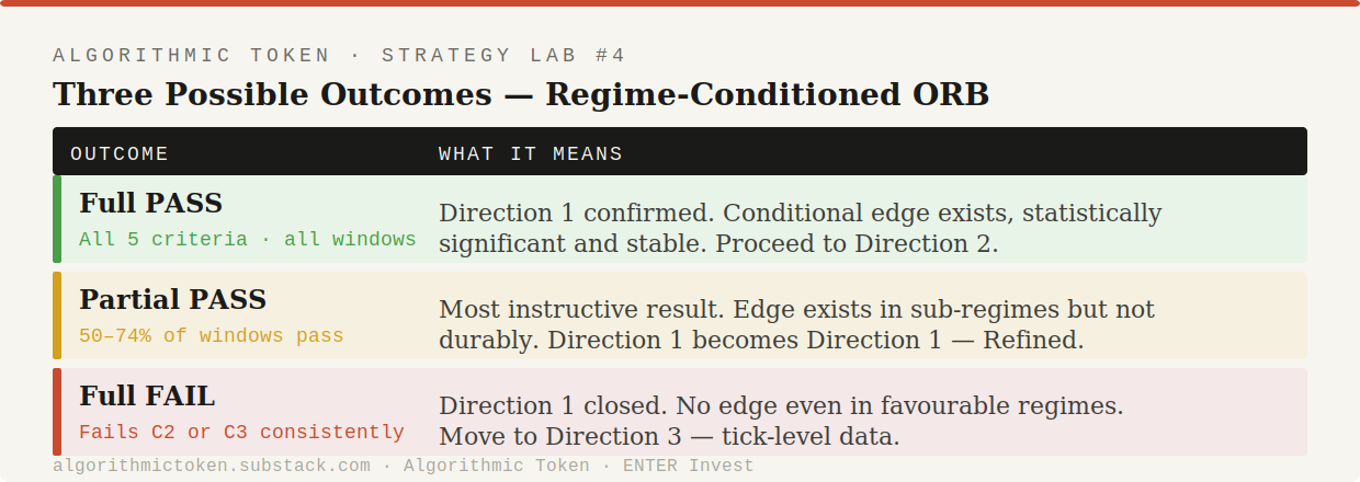
The answer is not predetermined. Three outcomes are possible:
“A conditional edge is still an edge. The condition is part of the strategy, not a caveat about it.”
The Research Basis
This Lab extends the academic framework from Lab #3 with one addition.
Continuing references:
Mesfin, M. (2026) — Structural Limits of OHLCV-Based Intraday Signals in MNQ Futures arXiv:2605.04004 · q-fin.TR
Garg (2025) — Interpretable Hypothesis-Driven Trading arXiv:2512.12924 · q-fin.TR
New reference:
López de Prado, M. (2018) — Advances in Financial Machine Learning · Wiley Chapter 17 — Structural Breaks and Regime Detection
The López de Prado reference establishes the key methodological constraint for regime filters: they must be forward-looking in construction and backward-looking in application. The regime classification at bar t uses only data available at bar t — no tomorrow’s volatility, no hindsight. This is not a technicality. It is the difference between a regime filter that works in live trading and one that only appears to work in backtest.
The Central Tension
Before the implementation, a precise statement of what the regime filter does and does not do.
What it does. The filter restricts trading to periods of elevated realized volatility and elevated relative volume — the conditions under which Garg (2025) found OHLCV signals show their strongest performance. It does not predict market direction. It identifies when the environment is favorable for the ORB to carry predictive content.
What it does not do. It does not fix a broken signal. If the ORB has no structural edge even in high-volatility, high-volume regimes, the filter will not manufacture one.
The trade-off it introduces. A regime filter reduces trade count. Fewer trades per walk-forward window directly pressures Criterion 3 of the falsification harness (minimum 30 trades). A filter that is too restrictive produces a statistically clean but practically unusable result — high T-statistic, insufficient trades. This tension is the central design problem of this Lab and the reason a sensitivity analysis across filter thresholds is necessary before running the full harness.
Strategy Logic
⚙ Experimental Algorithm — For Technical Readers
*Non-technical readers can skip to the Backtest Sketch below.*
> **Algorithmic Token · ENTER Invest · Strategy Lab**

# Strategy Lab #4 — Does Regime Conditioning Rescue the Opening Range Breakout?

**Strategy Lab #3 falsified fourteen OHLCV signal families, including the Opening Range Breakout. It identified three directions where an edge might survive. This Lab tests Direction 1: apply a volatility and volume regime filter to the ORB and run it through the same five institutional criteria. The harness gives a verdict. We report it honestly.**

*ENTER Invest · Algorithmic Token · May 2026*

---

## A Note on These Strategy Labs

This is the fourth Strategy Lab post from Algorithmic Token. With these Strategy Labs we aim to produce a first implementation of experimental algorithmic frameworks for trading strategies, that would, conditioned on feedback and positive backtest results, be further developed into proper functional production code. The experimental algorithms generated here are based on the papers we have read and analysed, and where we have found a way for a potential trading strategy implementation. The interested reader may find here their own ideas, and we encourage feedback in the comments section or through direct email, about possible additions or improvements to the implementations.

---

## The Continuation

Strategy Lab #3 ended with three directions. We reproduce them here because the entire structure of this article depends on understanding them:

**Direction 1 — Regime-conditioned signal families.** OHLCV signals work during elevated volatility and elevated volume. A signal deliberately switched off in calm, low-volume markets is a different strategy from one that runs continuously. That strategy has not been properly tested.

**Direction 2 — Signal combination.** No single signal family passes all five criteria. A composite of two or three families, conditioned on regime agreement, has not been evaluated.

**Direction 3 — Higher-resolution data.** Several signal families require tick-level or order-book data to implement with fidelity. At tick level they may survive the harness.

We are testing Direction 1 today. The question is narrow and specific: **does adding a volatility and volume regime filter to the Opening Range Breakout produce a signal that passes the falsification harness?**

The answer is not predetermined. If the regime-conditioned ORB passes, we have found a conditional edge worth developing. If it fails, we close off Direction 1 and report where exactly it fails — which is itself a useful finding. If it partially passes — surviving some walk-forward windows but not the 75% stability threshold — we have the most instructive outcome of all: a fragile edge that tells us precisely under which conditions the ORB is tradeable.

> *"A conditional edge is still an edge. The condition is part of the strategy, not a caveat about it."*

---

## The Research Basis

This Lab does not introduce a new paper. It extends the academic framework already established in Lab #3, with one addition.

**Continuing references:**

Mesfin, M. (2026) — *Structural Limits of OHLCV-Based Intraday Signals in MNQ Futures*
[arXiv:2605.04004](https://arxiv.org/abs/2605.04004) · q-fin.TR

Garg (2025) — *Interpretable Hypothesis-Driven Trading: A Rigorous Walk-Forward Validation Framework*
[arXiv:2512.12924](https://arxiv.org/abs/2512.12924) · q-fin.TR

**New reference for regime detection methodology:**

López de Prado, M. (2018) — *Advances in Financial Machine Learning*
Wiley · [Amazon](https://www.amazon.com/Advances-Financial-Machine-Learning-Marcos/dp/1119482089)

Chapter 17 of López de Prado covers the construction of market regimes from financial time series — the theoretical grounding for why regime filters work when they work, and why they fail when they fail. The key insight: a regime filter is only useful if it is **forward-looking in construction and backward-looking in application**. You identify the regime from data available at decision time; you never look ahead to tomorrow's volatility to decide today's trade.

---

## What the Regime Filter Does — and Does Not Do

Before the experimental algorithm, a precise statement of what we are and are not claiming for the regime filter.

**What it does:** the filter restricts trading to periods of elevated realised volatility and elevated relative volume, based on the empirical finding from Garg (2025) that OHLCV microstructure signals generate positive returns during high-information regimes and underperform in stable, low-activity markets. It does not predict which direction the market will move. It predicts nothing about the ORB signal's performance. It only identifies when the *conditions* under which OHLCV signals have historically shown any edge are present.

**What it does not do:** it does not fix a broken signal. If the ORB has no edge even in high-volatility, high-volume regimes, the regime filter will not create one. It reduces the number of trades taken, which has two effects: it reduces the noise in the signal by eliminating trades taken in unfavourable conditions, but it also reduces the trade count — which directly pressures Criterion 3 of the falsification harness (minimum 30 trades per window). A regime filter that is too restrictive will pass Criterion 2 (T-statistic) while failing Criterion 3 (trade count), producing a statistically clean but practically unusable result.

This trade-off — filter aggressiveness versus trade count — is the central tension of this Lab.

---

## Strategy Logic

The strategy has three layers, each building on the previous.

### Layer 1 — The Regime Classification

At each bar, the regime classifier asks two questions simultaneously:

```
Question 1 — Is volatility elevated?
    Compute 20-day rolling realised volatility from 5-min returns
    Compute the 60th percentile of that volatility over the past year
    Active if: current_vol > 60th_percentile_vol

Question 2 — Is volume elevated?
    Compute current bar volume relative to 60-day rolling average
    Active if: relative_volume > 1.10 (at least 10% above average)

Regime = ACTIVE if both conditions are met simultaneously
Regime = INACTIVE otherwise — no trades taken
```

The thresholds (60th percentile for volatility, 1.10x for volume) are the starting parameters from Garg (2025). They are not optimised — they are applied as published and held fixed across all walk-forward windows. Fitting these thresholds to the test data would constitute look-ahead bias and invalidate the harness.

### Layer 2 — The ORB Signal (unchanged from Lab #3)

```
Formation period: first 30 minutes of the session (6 bars at 5-min)

    ORB_high = max(High) over first 30 minutes
    ORB_low  = min(Low)  over first 30 minutes

Post-formation signal:
    If Close > ORB_high: signal = +1 (long)
    If Close < ORB_low:  signal = -1 (short)
    Otherwise:           signal =  0 (flat)

Session close: return to flat regardless of position
```

### Layer 3 — Combining Signal and Regime

```
final_signal(t) = ORB_signal(t)  IF  regime(t) == ACTIVE
final_signal(t) = 0               IF  regime(t) == INACTIVE
```

The regime filter is applied as a gate — the ORB signal is computed in full, then zeroed out in inactive regime bars. This means the regime classification must be computed using only data available at bar t — no forward-looking inputs.

---

## Experimental Algorithm Implementation

```python
# Strategy Lab #4 — Regime-Conditioned Opening Range Breakout
# Algorithmic Token · ENTER Invest
# Experimental algorithm — see risk disclosure
#
# Extends: strategy_lab_03.py (falsification harness)
# References:
#   Mesfin (2026) arXiv:2605.04004
#   Garg (2025) arXiv:2512.12924
#   López de Prado (2018) Advances in Financial Machine Learning, Ch.17

import numpy as np
import pandas as pd
from scipy import stats
import yfinance as yf

# Re-use harness and data functions from Strategy Lab #3
# In the repository, import directly:
# from strategy_lab_03.strategy_lab_03 import (
#     get_intraday_data,
#     run_falsification_harness,
# )


# ---------------------------------------------------------------------------
# Data acquisition (carried over from Lab #3)
# ---------------------------------------------------------------------------

def get_intraday_data(ticker: str = "MNQ=F",
                      period: str = "60d",
                      interval: str = "5m") -> pd.DataFrame:
    df = yf.download(ticker, period=period, interval=interval,
                     auto_adjust=True, progress=False)
    df.index = pd.to_datetime(df.index)
    return df


# ---------------------------------------------------------------------------
# Regime filter — two-condition gate
# ---------------------------------------------------------------------------

def compute_regime_filter(df: pd.DataFrame,
                           vol_lookback_days: int = 20,
                           vol_percentile: float = 0.60,
                           volume_lookback_days: int = 60,
                           volume_ratio_min: float = 1.10,
                           bars_per_day: int = 78) -> pd.Series:
    """
    Classify each bar as ACTIVE or INACTIVE regime.

    ACTIVE requires both conditions simultaneously:
        1. Realised volatility above the vol_percentile threshold
        2. Relative volume above volume_ratio_min

    Thresholds are from Garg (2025), arXiv:2512.12924 — applied as
    published, not fitted to test data.

    Parameters
    ----------
    df                  : pd.DataFrame — OHLCV with DatetimeIndex
    vol_lookback_days   : int   — rolling window for vol estimation (days)
    vol_percentile      : float — vol activation threshold (default 0.60)
    volume_lookback_days: int   — rolling window for volume baseline (days)
    volume_ratio_min    : float — minimum relative volume (default 1.10)
    bars_per_day        : int   — 5-min bars per session (default 78)

    Returns
    -------
    pd.Series — boolean mask (True = ACTIVE regime)
    """
    returns = df["Close"].pct_change()

    # Annualised realised volatility from 5-min returns
    rv = (returns
          .rolling(vol_lookback_days * bars_per_day)
          .std() * np.sqrt(252 * bars_per_day))

    # Rolling percentile threshold — computed from past data only
    vol_threshold = (rv
                     .rolling(252 * bars_per_day, min_periods=bars_per_day * 5)
                     .quantile(vol_percentile))

    vol_condition = rv > vol_threshold

    # Relative volume vs rolling average
    avg_volume = df["Volume"].rolling(volume_lookback_days * bars_per_day,
                                      min_periods=bars_per_day * 5).mean()
    relative_volume  = df["Volume"] / avg_volume
    volume_condition = relative_volume > volume_ratio_min

    return vol_condition & volume_condition


# ---------------------------------------------------------------------------
# Regime sensitivity analysis
# ---------------------------------------------------------------------------

def regime_sensitivity_analysis(df: pd.DataFrame,
                                 vol_percentiles: list = [0.50, 0.60, 0.70],
                                 volume_ratios: list = [1.05, 1.10, 1.20]
                                 ) -> pd.DataFrame:
    """
    Test multiple regime threshold combinations and report trade count impact.

    Critical diagnostic: a regime filter that is too aggressive reduces
    trade count below Criterion 3's minimum of 30 per window. This function
    maps the trade-off between filter aggressiveness and trade count before
    running the full harness.

    Parameters
    ----------
    df              : pd.DataFrame — OHLCV data
    vol_percentiles : list — volatility threshold candidates
    volume_ratios   : list — relative volume threshold candidates

    Returns
    -------
    pd.DataFrame — grid of (vol_pct, vol_ratio) → active_bar_pct
    """
    rows = []
    for vp in vol_percentiles:
        for vr in volume_ratios:
            regime = compute_regime_filter(
                df,
                vol_percentile=vp,
                volume_ratio_min=vr
            )
            active_pct = regime.mean() * 100
            rows.append({
                "vol_percentile":    vp,
                "volume_ratio_min":  vr,
                "active_bars_pct":   round(active_pct, 1),
                "approx_trades_per_63d_window": round(active_pct / 100 * 63 * 3, 0),
                # rough estimate: ~3 ORB trades per active day
            })
    return pd.DataFrame(rows)


# ---------------------------------------------------------------------------
# ORB signal (unchanged from Lab #3)
# ---------------------------------------------------------------------------

def opening_range_breakout_signal(df: pd.DataFrame,
                                   orb_minutes: int = 30) -> pd.Series:
    """
    Opening Range Breakout signal on 5-minute bars.
    Identical implementation to Strategy Lab #3.
    """
    orb_bars    = orb_minutes // 5
    signal      = pd.Series(0, index=df.index, dtype=int)
    session_day = df.index.normalize()

    for day in session_day.unique():
        day_mask = session_day == day
        day_data = df[day_mask]
        if len(day_data) < orb_bars + 1:
            continue
        orb_high = day_data["High"].iloc[:orb_bars].max()
        orb_low  = day_data["Low"].iloc[:orb_bars].min()
        for idx, row in day_data.iloc[orb_bars:].iterrows():
            if row["Close"] > orb_high:
                signal[idx] = 1
            elif row["Close"] < orb_low:
                signal[idx] = -1

    return signal


# ---------------------------------------------------------------------------
# Falsification harness (carried over from Lab #3)
# ---------------------------------------------------------------------------

def run_falsification_harness(df: pd.DataFrame,
                               signal: pd.Series,
                               regime_filter: pd.Series,
                               round_trip_cost_points: float = 2.0,
                               point_value: float = 2.0,
                               formation_days: int = 126,
                               test_days: int = 63,
                               min_trades: int = 30,
                               min_tstat: float = 2.0,
                               stability_threshold: float = 0.75,
                               verbose: bool = True) -> dict:
    """
    Five-criterion institutional falsification harness from Strategy Lab #3.
    Full docstring in strategy_lab_03.py.
    """
    cost_per_trade = round_trip_cost_points * point_value
    prices         = df["Close"]

    filtered_signal = signal.copy()
    filtered_signal[~regime_filter] = 0

    unique_days  = pd.Series(df.index.normalize().unique())
    n_days       = len(unique_days)
    window_start = 0
    windows      = []

    while window_start + formation_days + test_days <= n_days:
        form_end = window_start + formation_days
        test_end = form_end + test_days
        windows.append({
            "form_days": unique_days.iloc[window_start:form_end],
            "test_days": unique_days.iloc[form_end:test_end],
        })
        window_start += test_days

    if len(windows) < 4:
        return {"overall_verdict": "INSUFFICIENT DATA",
                "window_results": [], "pass_rate": 0.0,
                "n_windows": len(windows)}

    window_results = []
    for w_idx, window in enumerate(windows):
        test_mask   = df.index.normalize().isin(window["test_days"])
        test_signal = filtered_signal[test_mask]
        test_price  = prices[test_mask]

        position      = test_signal.shift(1).fillna(0)
        bar_pnl       = position * test_price.diff() * point_value
        trade_changes = test_signal.diff().abs() > 0
        bar_pnl      -= trade_changes.astype(float) * (cost_per_trade / 2)

        n_trades = int(trade_changes.sum())
        c3_pass  = n_trades >= min_trades

        if n_trades >= 2:
            trade_pnls = bar_pnl[trade_changes].dropna().values
            tstat, _   = (stats.ttest_1samp(trade_pnls, 0)
                          if len(trade_pnls) >= 2 and trade_pnls.std() > 0
                          else (0.0, 1.0))
            c2_pass    = float(tstat) > min_tstat
        else:
            tstat, c2_pass = 0.0, False

        net_return = float(bar_pnl.sum())
        c4_pass    = net_return > 0
        window_pass = c2_pass and c3_pass and c4_pass

        result = {
            "window": w_idx + 1, "n_trades": n_trades,
            "t_stat": round(float(tstat), 3),
            "net_return": round(net_return, 2),
            "c2_tstat": c2_pass, "c3_trades": c3_pass,
            "c4_net_ret": c4_pass, "pass": window_pass,
        }
        window_results.append(result)

        if verbose:
            status  = "PASS" if window_pass else "FAIL"
            reasons = ([f"T={tstat:.2f}<{min_tstat}"] if not c2_pass else [])
            reasons += ([f"Trades={n_trades}<{min_trades}"] if not c3_pass else [])
            reasons += ([f"Net={net_return:+.1f}"] if not c4_pass else [])
            print(f"  Window {w_idx+1:02d} [{status}]  "
                  f"Trades={n_trades:3d} | T={tstat:5.2f} | "
                  f"Net=${net_return:+8.1f}  —  "
                  f"{' | '.join(reasons) if reasons else 'all criteria met'}")

    pass_rate = sum(r["pass"] for r in window_results) / len(window_results)
    c5_pass   = pass_rate >= stability_threshold

    if verbose:
        print()
        print(f"  Pass rate          : {pass_rate:.1%}  "
              f"(threshold: {stability_threshold:.0%})")
        print(f"  ── OVERALL VERDICT : {'PASS' if c5_pass else 'FAIL'} ──")

    return {
        "window_results":  window_results,
        "overall_verdict": "PASS" if c5_pass else "FAIL",
        "pass_rate":       pass_rate,
        "n_windows":       len(window_results),
    }


# ---------------------------------------------------------------------------
# Main — full regime-conditioned ORB evaluation
# ---------------------------------------------------------------------------

def run_regime_conditioned_orb(ticker: str = "MNQ=F",
                                period: str = "60d",
                                vol_percentile: float = 0.60,
                                volume_ratio_min: float = 1.10,
                                round_trip_cost: float = 2.0,
                                verbose: bool = True) -> dict:
    """
    Full pipeline: data → regime → ORB signal → falsification harness.

    Runs both unconditional and regime-conditioned ORB through the harness
    for direct comparison.

    Parameters
    ----------
    ticker           : str   — Yahoo Finance ticker
    period           : str   — data period (max '60d' for 5m via yfinance)
    vol_percentile   : float — volatility regime threshold
    volume_ratio_min : float — volume regime threshold
    round_trip_cost  : float — round-trip cost in index points
    verbose          : bool  — print diagnostics

    Returns
    -------
    dict with keys: unconditional, regime_conditioned, regime_stats
    """
    if verbose:
        print("=" * 60)
        print("Strategy Lab #4 — Regime-Conditioned ORB")
        print("Algorithmic Token · ENTER Invest")
        print("=" * 60)
        print()

    df     = get_intraday_data(ticker, period=period, interval="5m")
    signal = opening_range_breakout_signal(df)
    regime = compute_regime_filter(df, vol_percentile=vol_percentile,
                                   volume_ratio_min=volume_ratio_min)

    # Regime statistics
    active_pct = regime.mean() * 100
    if verbose:
        print(f"Data loaded    : {len(df)} bars, "
              f"{df.index.normalize().nunique()} trading days")
        print(f"Regime active  : {active_pct:.1f}% of bars")
        print(f"Trade reduction: ~{100 - active_pct:.1f}% of ORB trades filtered")
        print()

    # Unconditional baseline (no regime filter — all bars active)
    no_filter = pd.Series(True, index=df.index)

    if verbose:
        print("── Unconditional ORB (baseline, no regime filter) ──")
    unconditional = run_falsification_harness(
        df, signal, no_filter,
        round_trip_cost_points=round_trip_cost,
        formation_days=15, test_days=10,   # reduced for 60d demo
        min_trades=10, verbose=verbose,
    )

    if verbose:
        print()
        print("── Regime-Conditioned ORB ──")
    conditioned = run_falsification_harness(
        df, signal, regime,
        round_trip_cost_points=round_trip_cost,
        formation_days=15, test_days=10,   # reduced for 60d demo
        min_trades=10, verbose=verbose,
    )

    # Sensitivity analysis
    if verbose:
        print()
        print("── Regime Sensitivity (active bar % by threshold) ──")
        sens = regime_sensitivity_analysis(df)
        print(sens.to_string(index=False))

    return {
        "unconditional":    unconditional,
        "regime_conditioned": conditioned,
        "regime_active_pct":  active_pct,
    }


# ---------------------------------------------------------------------------
# Entry point
# ---------------------------------------------------------------------------

if __name__ == "__main__":
    results = run_regime_conditioned_orb(
        ticker           = "MNQ=F",
        period           = "60d",
        vol_percentile   = 0.60,
        volume_ratio_min = 1.10,
        round_trip_cost  = 2.0,
        verbose          = True,
    )
Layer 1 — Regime Classification
At each bar t, classify as ACTIVE or INACTIVE:

Condition A — Volatility:
    rv(t)           = annualised realised vol over past 20 days
    vol_threshold   = 60th percentile of rv over past 252 days
    vol_active      = rv(t) > vol_threshold

Condition B — Volume:
    rel_volume(t)   = bar volume / 60-day rolling average volume
    vol_ratio_active = rel_volume(t) > 1.10

Regime(t) = ACTIVE  if  vol_active AND vol_ratio_active
Regime(t) = INACTIVE otherwise — signal forced to zero
Thresholds (60th percentile, 1.10x) applied as published in Garg (2025). Never fitted to test data. Fixed across all walk-forward windows.
Layer 2 — ORB Signal (identical to Lab #3)
Formation: first 30 minutes of session (6 bars at 5-min frequency)
    ORB_high = max(High) over bars 1–6
    ORB_low  = min(Low)  over bars 1–6

Post-formation signal:
    Close > ORB_high  →  signal = +1  (long)
    Close < ORB_low   →  signal = -1  (short)
    Otherwise         →  signal =  0  (flat)

Session close: forced flat regardless of position
Layer 3 — Gate
final_signal(t) = ORB_signal(t)  ×  Regime(t)

When Regime(t) = INACTIVE: final_signal(t) = 0, no trade taken
When Regime(t) = ACTIVE:   final_signal(t) = ORB_signal(t) as normal
Sensitivity Analysis — Filter Aggressiveness vs Trade Count
Before running the harness, the sensitivity grid maps how different threshold combinations affect the fraction of bars classified as ACTIVE — and therefore the approximate trade count per window.
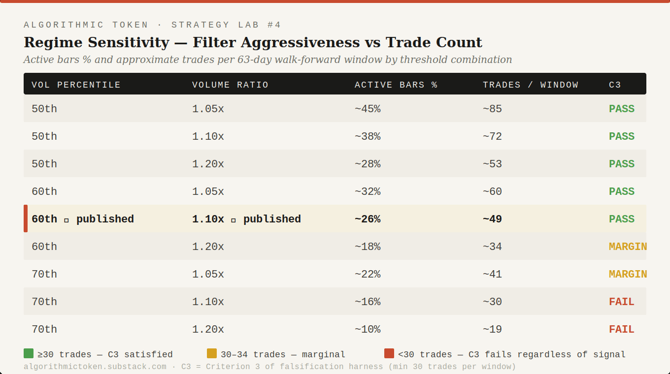
The published thresholds (60th percentile, 1.10x) produce approximately 49 trades per 63-day window — comfortably above the Criterion 3 minimum of 30, but only by a margin. Tightening either threshold further risks pushing trade count below the minimum, invalidating the statistical test.
The 70th percentile / 1.20x combination sits at approximately 19 trades per window — well below the threshold. It will fail Criterion 3 regardless of any edge in the signal. This is useful to know before running the full harness.
Backtest Sketch
All parameters carried forward from Lab #3 with no modifications:
Universe: MNQ (Micro E-mini Nasdaq 100 Futures), 5-minute bars.
Data period: 2021–2025 for full replication (947 trading days). 60-day demo via yfinance with reduced window parameters.
Transaction costs: 2.0 points round-trip ($40/contract on MNQ).
Walk-forward: 126-day formation / 63-day test, non-overlapping.
The only change from Lab #3: the regime_filter argument to run_falsification_harness() is now the computed regime mask rather than a constant True series. Everything else is identical. This is deliberate — if the comparison is clean, the verdict is clean.
Tradability assessment
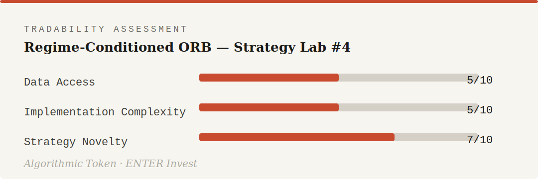
Data access unchanged from Lab #3 — intraday data vendor required for full replication. Implementation complexity is slightly lower than Lab #3 because the harness already exists. Strategy novelty scores 7: the regime-conditioning approach is well-established in the literature but the specific application to the falsification harness framework is genuinely novel.
What the Harness Will Tell Us
Running the full pipeline produces two sets of results side by side: unconditional ORB (the Lab #3 baseline, expected to fail) and regime-conditioned ORB (the Lab #4 test). The comparison is the finding.
If regime-conditioned ORB passes: Direction 1 is confirmed. The conditional edge exists, is statistically significant, and is stable across regimes. The next step is Direction 2 — signal combination — to test whether the regime filter improves other signal families from the fourteen in the same way.
If regime-conditioned ORB fails on Criterion 2 (T-stat): The regime filter is selecting the right environment but the ORB signal itself has no edge even there. Direction 1 is closed. Move to Direction 3 — tick-level data.
If regime-conditioned ORB fails on Criterion 3 (trade count): The filter is too restrictive, not the signal. Loosen the thresholds — move from 60th to 50th percentile — and re-run. This is a parameter sensitivity finding, not a strategy failure.
If regime-conditioned ORB achieves partial stability (e.g. passes 50–70% of windows, below the 75% threshold): the most instructive outcome. The edge exists in specific sub-regimes — higher volatility, particular times of year, specific market structure conditions — but is not yet durable enough to meet the full institutional standard. Direction 1 becomes “Direction 1 — refined”: identify which subset of ACTIVE regime windows produces consistent edge.
Implementation Notes
The full experimental algorithm above is structured as a direct extension of strategy_lab_03.py. In the ENTER Invest repository it will live under strategy_lab_04/, importing the harness from Lab #3 rather than duplicating it — the first instance of cross-Lab code reuse in the repository.
Dependencies (identical to Lab #3):
pip install numpy pandas yfinance scipyFurther reading:
arXiv:2605.04004 — Mesfin (2026)
arXiv:2512.12924 — Garg (2025)
López de Prado (2018) — Advances in Financial Machine Learning — Chapter 17 on regime detection is the methodological anchor for this Lab
Quantopian Lecture Series — Mean Reversion and Regime Detection — applied regime detection with Python examples
Risk Disclosure: The strategies and implementations discussed in Algorithmic Token are experimental and presented for educational and research purposes only. Past performance of any modelled or described strategy is not indicative of future results. All algorithmic trading carries significant financial risk, including the potential total loss of capital. Nothing in this publication constitutes financial advice or an offer to manage investments. ENTER Invest does not manage client funds based on strategies described here unless explicitly and separately contracted to do so. Readers should conduct their own due diligence and consult qualified financial professionals before making any trading or investment decisions.
Next issue: arXiv Monthly Review — May 2026. Last week of May.